Is the salesman travelling on foot or on an airplane?
This article describes an experiment to develop a version of the elastic net algorithm that works on spherical surfaces. I needed it for a computational neuroscience problem, but for those who are mainly interested in machine learning, it also serves a simple and intuitive demonstration of using gradient descent on non-Euclidian surfaces. The Tensorflow source code is available on GitHub. I also made a youtube video showing the algorithm in action.
The elastic net is a numerical algorithm for approximating the solution to the travelling salesman problem [1]. It’s an unsupervised learning algorithm that shares some of the features of Kohonen’s self-organizing map. In neuroscience, it’s typically used as a dimension reduction technique for modelling the development of topographic maps in the visual cortex [2]. In the traditional formulation of the travelling salesman problem, the cities that the salesman must visit are on a flat surface. That is assuming that the salesman is visiting cities confined to a relatively small region, so that the curvature of the Earth can be ignored. What if the salesman has to visit cities across the globe? I came up with the question when I was thinking about the mapping between the visual cortex and the retina, whose spherical geometry is very often ignored in neuroscience. But perhaps it would be interesting to take the spherical geometry into account?
Measuring distances on the sphere
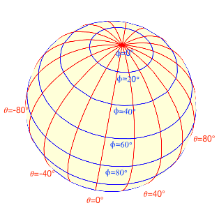
Before I explain the elastic net algorithm more formally, let’s consider a much simpler question: how do we move one spherical point $y$ to another fixed spherical point $x$, using gradient descent[3]? We might consider minimizing the Euclidian distance between the two, but then $y$ won’t stay on the surface. To force it stay on the sphere, we can use spherical coordinates $(θ, φ)$ to represent $x$ and $y$ (see Fig. 1), and use gradient descent to move $y$ around. This way, no matter how we change $θ$ and $φ$, $y$ always corresponds to a point on the sphere. However, calculating the distance requires some care. It’s not just the difference between the two coordinates. For example, the difference between $(θ, φ)=(10°, 20°)$ and $(20°, 20°)$ is 10°, which is the same as the difference between $(10°, 90°)$ and $(20°, 90°)$. However, the distance between the two points in the first case (near the north pole) is clearly much shorter than that of the second case (on the equator). There’s a lesson to be learned: the distance between two points is not always the difference of their coordinates (although this is the common practice in machine learning!).
The most straightforward way to measure distances on the sphere is to calculate the the geodesic distance - the arc length of the shortest path between the two points. But for reasons that will become more obvious later on, instead of minimizing the geodesic distance directly, we will maximize a function that is inversely proportional to the geodesic distance. This is accomplished by calculating $exp(\kappa , y \cdot x)$, where the dot product is calculated with the 3D cartesian coordinates of the two points, and $\kappa$ determines the concentration of the function. This formula is known as the 5-parameter Fisher-Bingham distribution, which is basically the Gaussian distribution of the sphere. I set $\kappa$ to 4.0 to give the function a broad distribution. I should note that the formula does not explicitly calculate the geodesic distance between $x$ and $y$. Instead, it depends on $y \cdot x$, which is the cosine of the geodesic distance.
Knowing how to measure distances solves only half of the problem
Now that we have an objective function that is based on geodesic distance, we can use gradient descent to update $(θ, φ)$, right? That can work, but it’s usually not the optimal solution. This is because knowing how far away two points are is only half of the problem. The second half of the problem is that the gradient also needs to respect the geometry of the sphere. Let’s take a look at an example.
Let’s say we want to move from (200°, 70°) to (70°, 40°). In Figure 2, the vector field is the gradient obtained by taking the derivatives of the Fisher-Bingham function with respect to $θ$ and $φ$. If we start at (200°, 70°) and follow the vector field, the path is illustrated by the green path. We do reach (70°, 40°), but the path length is 130.6°, which is about 35% longer than the geodesic distance between the two points, 97.3°. The gradient clearly is not correct. With the right gradient, we should be able to trace a path that is very close to the shortest path between the two points. The red path in Figure 2 is the result of gradient descent using the correct gradient. The path length is almost exactly the same as the optimal value.
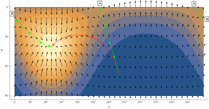
Figure 2: The color map illustrates the Fisher-Bingham distribution as a function of (θ, φ). The black arrows indicate the directions of the gradient, calculated by taking the derivative of the function with respect to θ and φ. To move from point (200°, 70°) to (70°, 40°), the green path is the solution obtained by following the black arrows, whereas the red path is the solution obtained by following the correct gradient (see the next section). The green path is continuous, but it is illustrated as 3 disjoint segments because the locations indicated by A and B are continuous on the sphere. Take a look at Figure 3 to see how the two paths look like on the sphere.
If you are eager to find out how the correct gradient is calculated, you can skip to the next section, but I think it’s worthwhile to understand what the green path means. The green path starts at (200°, 70°) and follows the gradient until it reaches point A at the top of the Figure 2. This is the north-pole, where all meridians converge, but since gradient descent treats θ and φ as variables in the Euclidean space, it continues to decrease $φ$ to make it a negative value (Figure 3). Luckily the Fisher-Bingham function is a periodic function defined to reflect the spherical geometry, so the green path immediately finds a hill to climb and ends up in (250°, -40°). Because we know spherical geometry, we interpret it as being the same point as our destination (70°, 40°). But to gradient descent, it is just another peak of the Fisher-Bingham function.
If this seems odd to you, it’s because we use an objective function based on spherical geometry, but the the way we calculate the gradient is Euclidean.
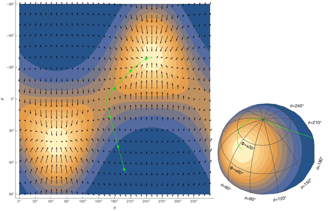
Figure 3: Left panel: The same Fisher-Bingham function as in Figure 2, except that the range of φ is expanded to -90°. Right panel: The Fisher-Bingham function plotted on the sphere. The panel on the left illustrates the Euclidean-space optimization problem for gradient descent. The panel on the right shows how the result is interpreted on the sphere.
Gradient descending with differential geometry
So how does the “correct gradient” look like? Can we plot it in Figure 2 for comparison? That’s the thing. We can’t, because the gradient does not live on the 2D space of Figure 2. Instead, the gradient vectors live in planes that are tangent to the spherical surface (Figure 4).

Figure 4: Left panel: The tangent planes to several points on the sphere. The red and the blue vectors represent the basis vectors of the tangent planes $(\hat{\theta},\hat{\phi})$. Right panel: The arrows illustrate the gradient of the Fisher-Bingham function (which is plotted by a blue-yellow color scale). Note that all the arrows are tangent to the spherical surface.
The correct way to calculate the gradient of a function defined on the sphere $f(\theta,\phi)$ can be easily found in textbooks and elsewhere (for example, MathWorld):
$$\nabla f = \frac{1}{sin\phi}\frac{\partial f}{\partial \theta}\hat{\theta} + \frac{\partial f}{\partial \phi}\hat{\phi}$$.
The ($\frac{\partial f}{\partial \theta},\frac{\partial f}{\partial \phi}$) part is just the gradient that we’ve seen in Figure 2. What this formula says is that there is nothing wrong with the gradient, it’s just that we have to interpret them as vectors on the tangent planes. The basis vectors of the tangent planes are $(\hat{\theta},\hat{\phi})$. You can look up the equations for calculating $(\hat{\theta},\hat{\phi})$ on MathWorld, but they are just the derivatives of the mapping between the spherical and the Cartesian coordinates. The left panel of Figure 4 plots $(\hat{\theta},\hat{\phi})$ as red and blue vectors. It also shows the tangent planes spanned by those basis vectors. What you can see from Figure 4 is that the changing orientation of the tangent plane is the mechanism for the gradients to reflect spherical geometry. For example, the tangent planes associated with points on different meridians converge at the north-pole.
Using the spherical gradient formula shown above, I calculated the gradient of the Fisher-Bingham function and plotted them as a vector field in the right panel of Figure 4. The red path is the the result of following the gradient from point (200°, 70°) to (70°, 40°) [4]. As mentioned before, it is very close to the great circle connecting the two points.
The elastic net in the Euclidean space
In the standard formulation of the elastic net, we are given a set of “prototypes” ($x_i$), and we use gradient descent to move another set of points $y_j$ to be as close to $x_i$ as possible. That doesn’t seem very difficult, but the crucial point is that associated with $y_j$ is a topography, meaning that there is a neighborhood relationship among the $y_j$’s, and we require that neighboring $y_j$’s are mapped onto points that are close to each other. Using the analogy of the traveling salesman, the prototypes $x_i$ are cities distributed on a 2D plane, and the order of the cities that he visits is the topology of $y_j$. The path has to be as short as possible, because traveling to a far away city is penalised. In the traveling salesman problem, the topology is 1D but most of the applications use the topography of a 2D grid (hence the elastic “net”).
The objective function for the standard elastic net is:
$E = -\alpha \kappa \sum_{i}^{} log \sum_{j}^{}\Phi(x_i, y_j, \kappa) + \frac{\beta}{2} \sum_{j}^{}\sum_{k \in N(j)}\Vert y_j - y_{k} \Vert^2$
where $N(j)$ is the neighbourhood of $y_j$, and
$\Phi(x_i, y_j, \kappa) = exp(\frac{-\Vert x_i - y_j \Vert^2}{2\kappa^2})$.
The second term is easy to understand. It’s just a regularization term requiring that neighboring points of $y_j$ are mapped to locations that are as close to each other as possible.
The first term is more tricky. It is for minimizing the distances between $x_i$ and $y_j$, but it uses a Gaussian $\Phi$ function to give heavier weights to nearby points. The width of $\Phi$ is dependent on $\kappa$, which is adjusted in the training process to cause the Gaussian to shrink. The procedure is similar to simulated annealing.
Intuitively, a $y_j$ is initialized to a random location, and it is moved in the training process under the influenced of two forces: it is attracted to $x_i$’s (especially to those that are nearby), and it is pulled by its neighbors. In the early stage of the training, the attracting forces of $x_i$’s are long-ranged, capable of dragging a large proportion of the net to its direction. But as the training continues, they become more local, capturing only the nearest $y_j$’s. This algorithm is Euclidean, because distance is measured by the norm of the difference vector.
The elastic net on the sphere
To adapt the algorithm to a context where the prototypes are on the sphere, we first need to rewrite the objective function such that distances are measured along the spherical surface. We already know how to rewrite the first term: we just replace the Gaussian with the Fisher-Bingham function that we’ve met earlier. For the second term, we should replace Euclidean distances with geodesic distances. The geodesic distance sounds complicated, but for the sphere, it is just $cos^{-1} (y_j \cdot y_k)$. Implementing this objective function is straightforward, but there is a small trick: the gradient of $cos^{-1}$ is unstable, because the derivative of $cos^{-1}$ becomes -∞ when $y_j$ and $y_k$ gets very close. It’s possible to replace $cos^{-1}$ with the more well-behaving $tan^{-1}$, but for this particular application, I simply clipped $y_j \cdot y_k$ to the range $(-1.0+\epsilon, 1.0-\epsilon)$ for a small positive $\epsilon$. This prevents the gradient from blowing up.
This video shows the elastic net learning to map the hemisphere. The red dots (N=200) are the prototypes, and the net is a 8x8 grid. The left panel shows the hemisphere in 3D. The right panel shows it in 2D using the area-preserving Lambert azimuthal projection.
In the early phase of the training, because the Fisher-Bingham functions are broad, the attracting forces of $x_i$’s act evenly on the $y_j$’s, causing the entire net to shrink to a small region. This behavior is very typical for elastic nets. But eventually the symmetry is broken, and the net unfolds. The rate at which $\kappa$ decreases is very important for the success of the algorithm. Many trials and errors are needed to find the right schedule.
This has been a simple demonstration, aiming to illustrate the basic principles of performing gradient descent in a context where geometry is important. I developed it to solve specific problems. The idea is generalized in a branch of mathematics called information geometry. As I programmed this algorithm, I was thinking… maybe it would be interesting to train neural networks to learn to measure distances on arbitrary manifolds, this neural network will need to take cartesian gradients as its inputs and transform them to reflect the underlying geometry…
References and Notes
- Note that it is different from “elastic net regularization” in regression analysis.
- Durbin R, Mitchison G (1990) A dimension reduction framework for understanding cortical maps. Nature 343 644-647. Durbin R, Willshaw D (1987) An analogue approach to the travelling salesman problem using an elastic net method. Nature 326 689-691. Goodhill GJ (2007) Contributions of theoretical modeling to the understanding of neural map development. Neuron 56, 301-311.
- This is, of course, the classical problem of finding the shortest path between two points on a differentiable manifold. The problem can be solved numerically or symbolically by solving a set of differential equations. We use gradient descent here, because it can be applied to a wider range of problems.
- There is a problem with the statement “following the gradient”. How do we move a point $y$ on the sphere according to the direction of the gradient, now that the gradient is pointing to a direction on the tangent plane, instead of to a point on the sphere? The proper way of doing it probably involves solving a differential equation, but I simply move the $y$ on the tangent plane (that is, off the spherical surface), and then project that point onto the sphere. It seems to work well.